2022년 10월 11일 화요일

[파인만 양자역학] 3-1. 진폭을 결합하는 법칙들 [1/2] (The laws for combining amplitudes)

[파인만 양자역학] 3-1. 진폭을 결합하는 법칙들 [1/2](The laws for combining amplitudes)

[참조]차교수의 물리 산책: 파인만 양자역학 3장/1강[강의]/[원문]
[처음][이전][다음]

[주의] ------------------------------------------------------------------------------------
파인만 양자역학을 내맘대로 번역하고 약간의 해설을 달아 봤습니다. 한글 해석과 덧붙인 [주]는 저의 개인적인 생각 이므로 그대로 받아 들이진 말아 주세요. 하지만 칭찬, 동의, 반론, 지적등 어떤 식으로든 의견은 환영 합니다.
-------------------------------------------------------------------------------------------

3. Probability Amplitudes
3장. 확률 진폭

3-1. The laws for combining amplitudes
3-1. 진폭을 결합하는 법칙들

When Schrödinger first discovered the correct laws of quantum mechanics, he wrote an equation which described the amplitude to find a particle in various places. This equation was very similar to the equations that were already known to classical physicists—equations that they had used in describing the motion of air in a sound wave, the transmission of light, and so on. So most of the time at the beginning of quantum mechanics was spent in solving this equation.

슈뢰딩거가 처음 양자역학에 맞는 법칙을 발견(discover!) 했을 때 그가 작성한 것은 거리상에 파동의 진폭[파동이 이동하는 경로상의 각지점에서 파동의 높이]를 기술하는 방정식이었다. 이 방정식은 고전 물리학에서도 익히 알려진 공기중에서 소리의 퍼짐이나 빛의 전파 같은 그런 방정식[시간에 대한 이차 미분 방정식]과 비슷했다. 그렇기 때문에 양자역학의 초창기 대부분은 이 방정식을 푸는데 시간을 보냈다.

[수학 문제를 풀면 뭔가 답이 나올거라는 희망을 품었다. 양자역학의 미시세계에 대한 새로운 개념은 쉽게 받아들이기 어려웠을 터이니 방정식이라도 풀고 싶었을 것이다.]

But at the same time an understanding was being developed, particularly by Born and Dirac, of the basically new physical ideas behind quantum mechanics.

하지만 [방정식에 메달리기와] 동시에 [양자역학의 개념의] 이해도 진행 되었다. 특히 보른, 디랙과 같은 이들은 양자역학에 내재된 새로운 물리학적 개념을 발전 시켰다.

[슈뢰딩거는 고전 물리학에서도 이미 알려진 파동의 방정식이 양자역학에도 적용될 수 있다는 것을 발견하였다. 보른, 디랙 같은 학자들은 이미 고전 물리학에서 거시세계의 자연현상을 설명하던 이차 미분 방정식이 미시세계에도 적용(물론 파동의 물리적인 현상이 아닌 확률진폭이라는 신개념으로 적용)될 수 있는 이유를 파헤치면서 양자 역학의 이론을 발전 시켰다.]

As quantum mechanics developed further, it turned out that there were a large number of things which were not directly encompassed in the Schrödinger equation—such as the spin of the electron, and various relativistic phenomena.

양자역학의 개념이 더 발전되자 슈뢰딩거 방정식과는 아무 관련이 없는 수많은 사항들이 등장하게 됐다. 일테면 전자의 스핀, 여러가지 상대론적인 현상들 등등.

[슈뢰딩거 파동 방정식은 그저 이차 미분 방정식으로 그 풀이는 파동이다. 이 풀이에 스핀이니 상대론적 현상 따위는 없다. 왜 파동의 진행 방향에서 위치와 시간의 함수가 확률 진폭이 되는지 그에 대한 궁금증을 풀려다 다른 양자역학 개념들이 파생되었다.]

Traditionally, all courses in quantum mechanics have begun in the same way, retracing the path followed in the historical development of the subject. One first learns a great deal about classical mechanics so that he will be able to understand how to solve the Schrödinger equation. Then he spends a long time working out various solutions. Only after a detailed study of this equation does he get to the “advanced” subject of the electron’s spin.

양자역학을 다루는 이전의 대부분 교육과정은 대동소이하게도 대개 역사적으로 거쳐왔던 경로를 따랐다. 고전역학에 많은 시간을 할애하여 학습을 한 후 슈뢰딩거 방정식을 어떻게 푸는지 해법을 이해하게 된다. 다양한 풀이법을 다루며 오랜시간을 투자했다. 이 방정식이 어떤 의미인지 자세히 살펴본 후에야 비로서 전자의 스핀이라는 "발전된" 화두에 도달하게 되었다.

[파동 방정식을 풀기 위해 고전 물리학에 몰입된 상태에서 마침내 슈뢰딩거 방정식을 풀고 이를 더 확대 발전 시킬 수 있는 "창의적" 사고를 했다는 점은 커다란 "발전"이다.]

We had also originally considered that the right way to conclude these lectures on physics was to show how to solve the equations of classical physics in complicated situations—such as the description of sound waves in enclosed regions, modes of electromagnetic radiation in cylindrical cavities, and so on. That was the original plan for this course.

우리는 처음에 고려했던 것은 이 물리학 강좌가 지향할(to conclude) 바른 방향은 다양한 조건에서 고전 물리학의 방정식들을 어떻게 푸는지 보여주는 거였다. 일테면 한정된 영역에서 음파의 기술이나 원통 통로(cavity)에서의 전자기 복사 방식 같은 그런 것이 이 강좌의 애초 목표였다.

However, we have decided to abandon that plan and to give instead an introduction to the quantum mechanics. We have come to the conclusion that what are usually called the advanced parts of quantum mechanics are, in fact, quite simple.

하지만 우리는 이 계획을 철회하기로 결정 했다. 그대신 양자역학 입문편을 하기로 했다. 우리가 고급 양자역학 이라고 하는 부분이 알고보면 아주 단순하다는 결론에 도달했기 때문이다.

---------------------------------------

The mathematics that is involved is particularly simple, involving simple algebraic operations and no differential equations or at most only very simple ones. The only problem is that we must jump the gap of no longer being able to describe the behavior in detail of particles in space.

[양자역학에 담긴] 수학은 특히 더 간단하다. 단순한 대수연산들을 포함할 뿐 미분 방정식은 없는데 있다고 해봐야 아주 단순하다. 유일하게 뛰어 넘어야할 틈이라면 공간상에 있는 입자를 세밀하게 기술할 능력이 없다는 점이다.

[벡터 미적분/미분방정식을 공부해 보자. 학교에서 성적 따려고 배울때 보다 심심풀이로 공부하기 좋은 강좌가 많다. 취미로 미적분과 미분방정식을 공부한다고 이야기 하면 멋지지 않나? 바로 양자역학을 취미로 공부한다고 하듯이.]

1. 미적분학-III/벡터 미적분
2. 공대생을 위한 미분 방정식

So this is what we are going to try to do: to tell you about what conventionally would be called the “advanced” parts of quantum mechanics. But they are, we assure you, by all odds the simplest parts—in a deep sense of the word—as well as the most basic parts. This is frankly a pedagogical experiment; it has never been done before, as far as we know.

그래서 지금부터 하려는 것이 이것이다. 이전에는 "고등" 양자역학이라고 했던 부분을 선보이려 한다. 하지만 이부분은 장담컨데 어딜 보더라도(by all odds) 기초편 만큼이나 말 그대로 단순하다[밑거나 말거나...]

In this subject we have, of course, the difficulty that the quantum mechanical behavior of things is quite strange. Nobody has an everyday experience to lean on to get a rough, intuitive idea of what will happen.

물론 우리는 이 과목에서 다루는 양자역학적 행동들을 받아들이기는 아주 어렵다. 누구도 무슨일이 벌어질지 개략적이거나 직감적인 생각을 일상 생활에서 경험한 사람은 없다.

[양자역학에서 다루는 미시세계의 현상을 거시세계에서 사는 사람으로써 경험해본 바도 없고 짐작도 못한다. 그러니 양자역학적 행동을 받아들이기 어려운 것이지 수학이 어려운 것이 아니다. 이해하지 못하겠으니 괜시리 '고등' 수학을 끄집어내서 힘들게 하는데 이는 '이상한' 물리학자들의 변명이 아닐까?]

So there are two ways of presenting the subject: We could either describe what can happen in a rather rough physical way, telling you more or less what happens without giving the precise laws of everything; or we could, on the other hand, give the precise laws in their abstract form.

그런데 이 주제를 다루는 두가지 길이 있다. 우리는 둘 모두를 취할 수 있다. 많든 적든 이 세상의 모든 법칙들을 세세히 동원하지 않고 좀더 물리학적인 측면에서 다루거나 좀더 추상화된 형식으로 구체적인 법칙들을 제시하는 방법도 있다.   

But, then because of the abstractions, you wouldn’t know what they were all about, physically. The latter method is unsatisfactory because it is completely abstract, and the first way leaves an uncomfortable feeling because one doesn’t know exactly what is true and what is false.

하지만 추상화로 인해 물리적인 의미를 완전히 파악하지 못하게 될 수도 있다. 후자의 방법은 너무나 추상적일 경우 만족스럽지 못할 수 있다. 그리고 전자의 경우 무엇이 맞는 말이고 무엇이 그른지 확실히 알지 못하기에 꺼림칙함을 남긴다.

['추상화'란 복합적 의미와 복잡한 절차를 한개의 상징으로 단순화 시키는 것을 말한다. 너무 고도로 추상화 수준에서 논하다보면 선문답이 될 수도 있다. 방정식 풀이에 집착하는 경우 막상 문제를 풀어 놓고도 그 의미를 깨닳지 못할 수 있다.]

We are not sure how to overcome this difficulty. You will notice, in fact, that Chapters 1 and 2 showed this problem. The first chapter was relatively precise; but the second chapter was a rough description of the characteristics of different phenomena. Here, we will try to find a happy medium between the two extremes.

우리는 이런 어려움을 어떻게 극복할지 확신이 없었다. 사실 여러분들은 1장과 2장에서 이 문제를 노출했었다는 점을 알아 챘을 것이다. 첫째 장은 상대적으로 구체성을 띄었다[여러 실험 상황을 제시하고 일일이 비교 설명함]. 하지만 둘째장은 서로다른 현상에 대해 개략적인 언급을 했었다[입자성과 파동성 관점의 차이]. 이제 두 극단에서 만족할 만한 중간선을 찾아보기로 하자.

We will begin in this chapter by dealing with some general quantum mechanical ideas. Some of the statements will be quite precise, others only partially precise. It will be hard to tell you as we go along which is which, but by the time you have finished the rest of the book, you will understand in looking back which parts hold up and which parts were only explained roughly.

이번 장은 양자역학의 일반적 개념을 다루는 것부터 시작해보자. 어떤 설명은 아주 구체적일 것이며 어떤 점은 상대적으로 느슨할 것이다. 어떤 면이 구체적이거나 구체적이지 않다고 일일이 말하긴 어렵겠지만 시간이 지나고 이 책의 마지막에 도달해서 되돌아보면 어느 부분이 끝까지 들고갈 내용이었고 어떤 부분이 임시로 개략적인 기술이었는지 깨닳게 될 것이다.

The chapters which follow this one will not be so imprecise. In fact, one of the reasons we have tried carefully to be precise in the succeeding chapters is so that we can show you one of the most beautiful things about quantum mechanics—how much can be deduced from so little.

이번 장에 이어질 장에서 다룰 내용은 결코 개략적이 아니다[이제 본격적으로 다룬다는 예고.] 사실 이후 장에서 조심스럽지만 세세히 다루려 하는 이유는 양자역학의 가장 아름다운 면을 보여주려고 하기 때문이다. 작은 것에서 얼마나 커다랗게 뻗어나갈지 기대해보라.

--------------------------------

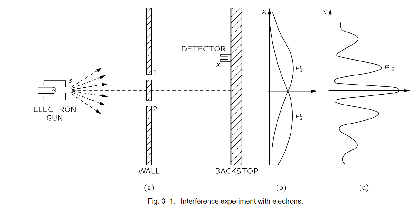
We begin by discussing again the superposition of probability amplitudes. As an example we will refer to the experiment described in Chapter 1, and shown again here in Fig. 3–1. There is a source s of particles, say electrons; then there is a wall with two slits in it; after the wall, there is a detector located at some position x.

확율진폭의 중첩을 다시 꺼내 논의를 시작해보자. 예로 그림 3-1에 보인 것 처럼 1장에서 기술한 실험을 참조하겠다. 전자 입자의 출발지를 s 라 하고 중간에 두개의 구멍이 뚫린 벽이  있으며 벽을 지나 도착지의 어느 지점 x 에 검지기가 놓였다.  

We ask for the probability that a particle will be found at x. Our first general principle in quantum mechanics is that the probability that a particle will arrive at x, when let out at the source s, can be represented quantitatively by the absolute square of a complex number called a probability amplitude—in this case, the “amplitude that a particle from s will arrive at x.”

위치 x 지점에서 한 입자가 발견될 확률을 구하려 했다. 우리가 접한 양자역학의 첫번째 일반 원리는 출발점 s를 떠난 입자가 x 지점에 도달할 가능성이 어느 정도 인지 정량적으로 나타내는 것[확율] 이었다. 이 확률은 확률진폭이라고 하는 복소수를 제곱하여 절대값을 취해 구할 수 있다는 것이었다. 그러니까 "s 를 떠나 x에 도착할 입자의 확률 진폭"이라고 하면 되겠다.

[확율 분포가 마치 파동의 간섭의 현상과 같은 양상을 띌 뿐이지 실제로 입자가 파동의 운동을 한다는 뜻이 아니다.]

We will use such amplitudes so frequently that we will use a shorthand notation—invented by Dirac and generally used in quantum mechanics—to represent this idea. We write the probability amplitude this way:

앞으로 이러한 표현이 매우 빈번히 나올 것이므로 좀 간략히 표기하기로 하자. 디랙(Dirac)에 의해 고안되어 양자역학 분야에서 [확률 진폭의] 개념을 나타내기 위해 널리 사용된 표기법이다. 이제 확률진폭은 아래와 같이 표기한다.

    ⟨Particle arrives at | particle leaves s    ................................    (3.1)

In other words, the two brackets ⟨⟩ are a sign equivalent to “the amplitude that”; the expression at the right of the vertical line always gives the starting condition, and the one at the left, the final condition.

다른 말로 하면 두 브라켓 <>은 "~과정을 거친 진폭" 이라는 뜻을 표현한다. 이런 표현은 가운데 수직선을 두고 오른편이 출발점의 조건을 나타내며 왼편은 최종지의 상황을 나타낸다.

[복잡한 과정을 거친 복합적인 의미를 간략히 상징화 하는 것을 '추상화'라고 한다. 브라켓 <>는 출발지의 조건과 도착지에서 입자가 발견될 확률진폭을 단순하게 상징화 했다.]

Sometimes it will also be convenient to abbreviate still more and describe the initial and final conditions by single letters. For example, we may on occasion write the amplitude (3.1) as

출발지 조건과 도착지 상황을 알파벳 문자 한개로 표현하면 좀더 편할 것이다. 예를 들어 진폭 (3.1)을 다음과 같이 쓴다.

    ⟨x|s⟩    ...................................    (3.2)

We want to emphasize that such an amplitude is, of course, just a single number—a complex number.

그렇게 영문자 한개로 표현하긴 했지만 당연히 복소수로서 진폭을 나타낸 것이란 점을 강조해 둔다.

We have already seen in the discussion of Chapter 1 that when there are two ways for the particle to reach the detector, the resulting probability is not the sum of the two probabilities, but must be written as the absolute square of the sum of two amplitudes. We had that the probability that an electron arrives at the detector when both paths are open is

이미 1장에서도 봤지만 검지기에 도달하기 까지 입자에게는 두가지 길이 있고 두 경로를 지난 확율의 합은 각 경로를 지난 확율의 합과 같지 않다. 그렇더라도 [두 구멍을 열어놓음] 최종 확율은 두 [확율]진폭의 합에 절대값 제곱으로 표현되어야 한다. 두개의 경로를 열어놓고 감지기에 도착할 전자의 확율은 다음과 같이 얻는다.

    P_12 = |ϕ_1 + ϕ_2|^2    ..............................    (3.3)

We wish now to put this result in terms of our new notation. First, however, we want to state our second general principle of quantum mechanics: When a particle can reach a given state by two possible routes, the total amplitude for the process is the sum of the amplitudes for the two routes considered separately. In our new notation we write that

이제 이 결과를 새로운 표기법으로 표현해 보고자 한다. 먼저 그전에 양자역학의 두번째 일반 원리를 되새겨 본다. 입자가 거치게 될 경로가 두개라고 할 때, 총 진폭은 각 경로를 개별적으로 구한 진폭의 합하는 방식으로 구한다.

    ⟨x|s⟩_both holes open = ⟨x|s⟩_through_1 + ⟨x|s⟩_through_2    ................    (3.4)

Incidentally, we are going to suppose that the holes 1 and 2 are small enough that when we say an electron goes through the hole, we don’t have to discuss which part of the hole. We could, of course, split each hole into pieces with a certain amplitude that the electron goes to the top of the hole and the bottom of the hole and so on.

부연해서 설명해 둘 점은 구멍 1과 2는 전자 하나가 통과할 정도로 충분히 작다고 가정하고 구멍의 어느 부분에 닿는지에 대해선 고려하지 않겠다. 물론 전자가 한 구멍의 윗부분과 다른 구멍의 아랫부분 사이를 특정 진폭을 고려해 분리해 놓을 수 있다는 등의 고려사항이 가능 하다고 하놓겠다. [구멍의 물리적 형상으로 인해 전자의 경로가 변경될 수 있다는 점은 고려하지 않겠다.]

We will suppose that the hole is small enough so that we don’t have to worry about this detail. That is part of the roughness involved; the matter can be made more precise, but we don’t want to do so at this stage.

우리는 구멍이 충분히 작아서 구멍에 대한 세세한 영향에 대해서 고려하지 않기로 하겠다. 이는 간략화 하는 면이 있는데 더 정밀하게 취급할 요인이지만 지금 단계에서는 그렇게 하진 않겠다.

Now we want to write out in more detail what we can say about the amplitude for the process in which the electron reaches the detector at x by way of hole 1. We can do that by using our third general principle: When a particle goes by some particular route the amplitude for that route can be written as the product of the amplitude to go part way with the amplitude to go the rest of the way.

이제 전자가 구멍 1을 통과한 후 x 지점에 놓인 검지기에 도달하는 과정을 좀더 구체적으로 기술하려고 한다. 이 시점에서 세번째 일반 원리를 적용한다. 입자가 특정 경로를 지날때 그 경로상의 진폭은 거쳐간 부분 구간의 진폭의 곱으로 표현한다.

[양자역학을 다룰 때  확율진폭 계산을 위한 계산법으로써 도입한 세가지 일반 원리(general principle)를 정의한다. 첫번째, 확율진폭은 복소수로 표현하고 진폭 값은 절대값의 제곱하여 구한다. 이 진폭값을 브라켓 표기법을 활용 하겠다. 두번째, 입자가 통과 할 경로가 여럿일 경우 총 확율 진폭은 각 경로의 확율 진포의 합으로 구한다. 세번째, 전자가 지나갈 한 경로가 부분적으로 나뉠 경우 그 경로의 확율진폭은 각 부분 경로의 확율진폭의 곱으로 구한다. 확율진폭의 덧셈과 곱셈의 의미는 나중에 따져보기로 하고 일단 원리로써 정리해 둔다.]

For the setup of Fig. 3–1 the amplitude to go from s to x by way of hole 1 is equal to the amplitude to go from s to 1, multiplied by the amplitude to go from 1 to x.

그림 3-1과 같은 실험 구조에서 전자의 근원(출발)지 s에서 구멍 1을 지나 x에 이르는 경로의 [확률]진폭은 s에서 구멍 1까지의 진폭과 구멍 1에서 x에 이르는 진폭의 곱과 같다.

     ⟨x|s⟩_via_1 = ⟨x|1⟩⟨1|s⟩    ................................ (3.5)

Again this result is not completely precise. We should also include a factor for the amplitude that the electron will get through the hole at 1; but in the present case it is a simple hole, and we will take this factor to be unity.

다시 짚어 두지만 이 결과는 사실 완전하진 않다[모든것을 세세히 따진게 아니다.] 전자가 구멍 1을 지나는 동안 받을 영향도 고려해야 하지만 지금으로서는 구멍을 단순화 했고 구멍의 영향은 차치해(to be unity) 두기로 한다.

You will note that Eq. (3.5) appears to be written in reverse order. It is to be read from right to left: The electron goes from s to 1 and then from 1 to x.

식 (3.5)에 기술된 표현을 보면 순서가 뒤집어 진것처럼 보일 것이다. 오른쪽에서 왼쪽으로 읽어야 하는데, 전자가 진행한 경로는 s 에서 1로, 이어서 1에서 x가 된다.

In summary, if events occur in succession—that is, if you can analyze one of the routes of the particle by saying it does this, then it does this, then it does that—the resultant amplitude for that route is calculated by multiplying in succession the amplitude for each of the successive events.

요약하면 만일 사건이 연속적으로 일어나는경우, 그러니까 분석을 통해 입자가 지나간 경로를 이곳을 거치고 이어서 이곳을 거쳤다고 말할 수 있다면  연속된 각 사건의 진폭을 연속적으로 곱해 최종 진폭을 계산할 수 있다.

Using this law we can rewrite Eq. (3.4) as

이 법칙[확율진폭 곱의 원리]를 적용해 식 (3.4)를 다시 쓰면 다음과 같다.

    ⟨x|s⟩_both = ⟨x|1⟩⟨1|s⟩ + ⟨x|2⟩⟨2|s⟩.

---------------------------------------------------------------

Now we wish to show that just using these principles we can calculate a much more complicated problem like the one shown in Fig. 3–2. Here we have two walls, one with two holes, 1 and 2, and another which has three holes, a, b, and c. Behind the second wall there is a detector at x, and we want to know the amplitude for a particle to arrive there.

이 [확률진폭 연산의] 원리들을 이용하여 그림 3-2와 같이 좀더 복합적인 구성을 갖는 문제에 적용해 보자. 이 구성에는 두개의 벽이 있고 그중 한 벽에 두 구멍이 뚫렸는데 각각 1과 2라고 하자. 또다른 벽에는 각각 a, b, c 라는 이름을 붙인 세개의 구멍이 뚫려있다. 두번째 벽 뒤의 벽에 x 지점에 검지기가 놓여있다. 이 검지기에 도착할 입자의 확률진폭을 구하고자 한다.

Well, one way you can find this is by calculating the superposition, or interference, of the waves that go through; but you can also do it by saying that there are six possible routes and superposing an amplitude for each. The electron can go through hole 1, then through hole a, and then to x; or it could go through hole 1, then through hole b, and then to x; and so on.

그럼 이 총 진폭은 입자가 통과하는 구간마다 중첩 혹은 간섭을 계산하여 구할 수 있다. 하지만 조합가능한 경로가 여섯가지나 되고 각 구간마다 진폭을 구해 합쳐야 한다. 전자는 구멍 1을 통과한 후 이어 구멍 a를 통과하여 x 에 도착할 수 있다. 또는 구멍 1을 통과한 후 구멍 b를 통과하여 x 에 도달할 수도 있다. 그런식으로 여러 조합이 가능하다. 

According to our second principle, the amplitudes for alternative routes add, so we should be able to write the amplitude from s to x as a sum of six separate amplitudes. On the other hand, using the third principle, each of these separate amplitudes can be written as a product of three amplitudes.

경로가 다른 경우 더하기로 한 두번째 확률진폭 계산의 원리에 따라 s 에서 시작하여 x 에 도달하기까지 총 확률진폭은 여섯가지의 개별 경로별 진폭을 모두 더하여 구한다. 한편, 각 경로별 진폭은 세 부분 구간의 진폭을 [전자가 이동하는 경로상 순서에 따라] 곱하여 독립적으로 구한다.

For example, one of them is the amplitude for s to 1, times the amplitude for 1 to a, times the amplitude for a to x.

예를들어 여섯개 경로중 한 경로의 확률진폭은 s에서 1로 가는 진폭 곱하기 1에서 a 로 가는 진폭 곱하기 a 에서 x 까지의 진폭을 곱한다.

Using our shorthand notation, we can write the complete amplitude to go from s to x as

간략한 [브라켓] 표기법을 적용하여 s 에서 x 까지의 총 진폭을 구하는 식을 포현하면 다음과 같다.  

    ⟨x|s⟩ = ⟨x|a⟩⟨a|1⟩⟨1|s⟩ + ⟨x|b⟩⟨b|1⟩⟨1|s⟩ + ⋯ + ⟨x|c⟩⟨c|2⟩⟨2|s⟩.

We can save writing by using the summation notation

이렇게 모두 더하기로 나열하기 보다 총합 기호를 쓰면 간략해보이기도 하고 그럴듯 하다.

    ⟨x|s⟩ = ∑i=1,2α=a,b,c(⟨x|α⟩⟨α|i⟩⟨i|s⟩)    .........................    (3.6)

In order to make any calculations using these methods, it is, naturally, necessary to know the amplitude to get from one place to another. We will give a rough idea of a typical amplitude. It leaves out certain things like the polarization of light or the spin of the electron, but aside from such features it is quite accurate.

이런 식으로 계산을 하려면 당연히 한곳에서 다른곳에 이르는 진폭을 알아야야 할 것이다. 기초적인 확률진폭 계산법을 개략적으로 다뤄볼 것이다. 일테면 빛의 편광 이나 전자의 스핀 같은 아주 세밀한 요소들은 잠시 접어두기로 한다.

[세밀한 요소들은 경로상 영향을 주는 요인이므로 세번째 원리에 따라 그로 인한 진폭을 곱해주면 된다. 편광, 스핀 같은 입자에 내재한 특성들 역시 간섭과 같이 입자가 진행하며 어디에 위치할지 영향을 주는 요인들로  취급된다.]

---------------------------------------------------------------------------------------------------
[참고]
1. 차교수와 물리산책[링크]
3. 차교수의 물리 산책: 파인만 양자역학 3장/1강[강의]/[원문]


2022년 10월 8일 토요일

[파인만 양자역학] 2-6. 철학적 함의(Phylosophical implications)

[파인만 양자역학] 2-6. 철학적 함의(Phylosophical implications)


[참조]차교수의 물리 산책: 파인만 양자역학 2장/[원문]
[처음][이전][다음]

[주의] ------------------------------------------------------------------------------------
파인만 양자역학을 내맘대로 번역하고 약간의 해설을 달아 봤습니다. 한글 해석과 덧붙인 [주]는 저의 개인적인 생각 이므로 그대로 받아 들이진 말아 주세요. 하지만 칭찬, 동의, 반론, 지적등 어떤 식으로든 의견은 환영 합니다.
-------------------------------------------------------------------------------------------

Chapter 2. The relation of wave and particle viewpoints)
2장. 파동과 입자 관점의 차이

2–6. Philosophical implications
2-6. 철학적 함의(Phylosophical implications)

Let us consider briefly some philosophical implications of quantum mechanics. As always, there are two aspects of the problem: one is the philosophical implication for physics, and the other is the extrapolation of philosophical matters to other fields.

양자역학이 가지는 철학적 함의를 간략하게 집어 보자. 늘 그랬던 것처럼 질문에는 양면이 있다. 먼저 물리학에 담긴 철학적 의미와 그 다음으로 [물리학 이외의] 다른 영역에 철학적 의미와 상관성이다.

When philosophical ideas associated with science are dragged into another field, they are usually completely distorted. Therefore we shall confine our remarks as much as possible to physics itself.

과학과 관련된 철학적 개념(idea)이 다른 영역으로 끌려 들어 가면서(drag into ~) 딴판으로 왜곡되곤 한다. 따라서 우리의 논의를 물리학의 영역에 힘껏 붙잡아 둬야 한다. 

First of all, the most interesting aspect is the idea of the uncertainty principle; making an observation affects the phenomenon. It has always been known that making observations affects a phenomenon, but the point is that the effect cannot be disregarded or minimized or decreased arbitrarily by rearranging the apparatus.

먼저, 가장 흥미를 끄는 측면은 관찰(observation)이 현상(phenomenon)에 영향을 미칠 거라는 불확정성 원리의 개념이다. 관측하는 것으로 현상[발현]에 영향을 미친다고 들 알려져 있다. 하지만 요점은 그 영향이라는 것이 [측정] 장치들을 재배치 하는 것으로 없앤다거나 최소화 시키거나 임의로 줄일 수 없다는 점이다.

[관측으로 인해 결과가 바뀐다고 하지만 관측 방법(장치의 재배치)을 바꾼다고 결과에 영향을 주지 않았다. 그렇다면 관측이 결과에 영향을 미친다는 생각은 유효한가?]

When we look for a certain phenomenon we cannot help but disturb it in a certain minimum way, and the disturbance is necessary for the consistency of the viewpoint. The observer was sometimes important in prequantum physics, but only in a trivial sense.

우리가 어떤 현상을 관찰할 때 영향을 최소화 하긴 하겠지만 피할 수는 없고 일관된 관점을 위해서는 이런 '개입'은 필수다. 양자물리학 이전에(pre-quantum) 관찰자는 때로 매우 중요했으나 대개 무시되곤 했다.

The problem has been raised: if a tree falls in a forest and there is nobody there to hear it, does it make a noise? A real tree falling in a real forest makes a sound, of course, even if nobody is there. Even if no one is present to hear it, there are other traces left. The sound will shake some leaves, and if we were careful enough we might find somewhere that some thorn had rubbed against a leaf and made a tiny scratch that could not be explained unless we assumed the leaf were vibrating. So in a certain sense we would have to admit that there is a sound made.

이런 문제를 상정해보자. 숲에서 나무가 쓰러졌으나 그것을 듣는 이가 아무도 없었다고 해보자. 그렇다면 [쓰러지는] 소리가 났었다고 할 수 있을까? 실제로 나무는 쓰러졌고 소음도 일었지만 듣는이가 아무도 없었을 뿐이다. 그 소리를 들었다는 사람이 아무도 없었더라도 다른 흔적(traces)은 남아 있다. 자세히 살펴 보면 가시(thorn)가 나뭇잎을 비벼서(rubbed) 작은 상처(scratch)를 냈는데 그 상처는 나뭇잎을 흔렸기 때문이라는 이유말고는 설명할 수 없다. 따라서 소음이 났다는 것을 어떤 식으로든 받아들여야 할 것이다.

We might ask: was there a sensation of sound? No, sensations have to do, presumably, with consciousness. And whether ants are conscious and whether there were ants in the forest, or whether the tree was conscious, we do not know. Let us leave the problem in that form.

이런 의문을 가질 수 있다. 소리의 감응[소리에 대한 반응]이 있었을까? 그렇지 않다. 추측컨데 감응은 인지했을 때 일어난다. 만일 숲어딘가에 있던 개미가 인지했을 지도 모를 지언정 우리는 인지하지 못했다. 이제 이 문제는 그대로 놔 두자.

Another thing that people have emphasized since quantum mechanics was developed is the idea that we should not speak about those things which we cannot measure. (Actually relativity theory also said this.) Unless a thing can be defined by measurement, it has no place in a theory. And since an accurate value of the momentum of a localized particle cannot be defined by measurement it therefore has no place in the theory. The idea that this is what was the matter with classical theory is a false position. It is a careless analysis of the situation. Just because we cannot measure position and momentum precisely does not a priori mean that we cannot talk about them. It only means that we need not talk about them.

또다른 문제는 양자역학이 대두되자 사람들은 우리가 측정할 수 없는 것은 언급하지 말아야 한다는 사상을 강조했다는 점이다. (실제로 상대론도 이에 동조했었다.) 측정(관찰)로 실체를 정의할 수 없다면 이론이 설 자리는 없다. 입자의 위치를 특정할 수 없기에 운동량의 정확한 값을 측정할 수 없으므로 이론이 성립할 여지가 없다. 이 생각이 바로 고전물리학이 어긋나게된 문제의 지점이다. 상황에 대한 분석이 세심하지 못했다. 그저 위치와 운동량을 정확히 측정할 수 없다는 점이 우리가 논의할 수도 없다고 말하는 가장 우선적인 이유가 될 수 없다. 언급할 필요가 없을 뿐이다. [특정 할 수 없다는 점을 만하지 말고 현상은 인정하자.]

The situation in the sciences is this: A concept or an idea which cannot be measured or cannot be referred directly to experiment may or may not be useful. It need not exist in a theory. In other words, suppose we compare the classical theory of the world with the quantum theory of the world, and suppose that it is true experimentally that we can measure position and momentum only imprecisely. The question is whether the ideas of the exact position of a particle and the exact momentum of a particle are valid or not.

과학계의 상황은 이랬다. 실험으로 직접 측정될 수 없는 개념 또는 생각은 유효하지도 않고 유효할 수도 없다는 것이다. 그런 생각은 이론으로 존재할 필요도 없다. 달리 말하면, 고전물리 이론이 통하는 세계와 양자이론의 세계를 비교한다고 해보자. 우리가 위치와 운동량을 개략적으로 만 실험으로 측정할 수 있다고 해보자. 이때 해야할 질문은 입자의 정확한 위치와 정확한 운동량이 있다는 생각이 유효한지 또는 아닌지다. [양자현상은 있으나 위치와 운동량을 각각 특정할 수 없다고 불확정성 원리라는 생각을 부정할 일은 아니다.]

The classical theory admits the ideas; the quantum theory does not. This does not in itself mean that classical physics is wrong. When the new quantum mechanics was discovered, the classical people—which included everybody except Heisenberg, Schrödinger, and Born—said: “Look, your theory is not any good because you cannot answer certain questions like: what is the exact position of a particle?, which hole does it go through?, and some others.”

고전 이론에서는 그렇게 [실험으로 입증되어야 한다고] 받아들였고 양자이론은 그러지 않았다. 고전물리학이 틀렸다는 게 아니다. 새로 양자역학이 등장 했을 때 하이젠버그, 슈뢰딩거 그리고 보른을 제외한 대부분 고전역학계 사람들은 이렇게 말했다. "봐라, 당신들 이론이 제대로 된게 없어. 당신들은 입자의 정확한 위치 조차 대답하질 못하잖아? 입자가 어느 구멍으로 통과 했는지 알아? 그외에도 한둘이 아니지."  

Heisenberg’s answer was: “I do not need to answer such questions because you cannot ask such a question experimentally.” It is that we do not have to.

하이젠버그의 대답은 이랬다. "당신들은 그 의문을 실험적으로 제시하지 못했으니 나는 그 질문에 답할 필요가 없군요." 그것이 바로 우리가 하면 않되는 질문이다.

Consider two theories (a) and (b); (a) contains an idea that cannot be checked directly but which is used in the analysis, and the other, (b), does not contain the idea.

(a) 와 (b)라는 두개의 이론이 있다고 해보자. (a)라는 이론은 즉시 확인할 수는 없지만 분석(해석)의 과정에서 활용될 수 있고, 다른 이론 (b)는 그 개념을 가지고 있지 않다.

[(a)라는 이론에 담긴 개념을 설명 할 수 없기 때문에 틀렸다고 주장한다. 실체를 직접 확인할 수 없는 개념은 받아들일 수 없다는 것이다.]

If they disagree in their predictions, one could not claim that (b) is false because it cannot explain this idea that is in (a), because that idea is one of the things that cannot be checked directly.

만일 두 이론의 예측이 일치하지 않다면 (a)라는 이론에 담긴 개념을 설명할 수 없다고 해서 (b)라는 이론이 틀렸다고 주장하면 않될 것이다. 그 개념도 직접 설명 될 수 없는 여러 개념들 중 하나이기 때문이다.

It is always good to know which ideas cannot be checked directly, but it is not necessary to remove them all. It is not true that we can pursue science completely by using only those concepts which are directly subject to experiment.

어떤 개념은 직접 확인될 수 없다는 것을 늘 인지하고 있어야 한다. 하지만 모두 제거할 필요는 없다[어떤 개념이 직접 확인 할 수 없다고 해서 깡그리 무시될 필요는 없다는 점을 필히 염두에 두어야 한다.] 실험으로 직접 확인될 수 있는 개념만이 우리가 추구할 과학이라고 여기는 것은 옳지않다.

In quantum mechanics itself there is a probability amplitude, there is a potential, and there are many constructs that we cannot measure directly. The basis of a science is its ability to predict. To predict means to tell what will happen in an experiment that has never been done. How can we do that?

양자역학 스스로 확률 진폭이라는 개념을 가지고 있고, 가능성을 말하며 직접 확인할 수 없지만 여러 구성들[입자의 현상을 설명할 수 있는 이론들]을 가지고 있다. 예측할 수 있는 능력은 과학의 기본이다. 예측이란 이제까지 없었던 어떤 일이 벌어질지 실험으로 말하는 것이다. 어떻게 할 수 있을까?

By assuming that we know what is there, independent of the experiment. We must extrapolate the experiments to a region where they have not been done. We must take our concepts and extend them to places where they have not yet been checked.

실험으로 얻어지지는 않았더라도 이전에 있었던 경험을 취합하자. 이제까지 없었던 영역으로 실험을 추론해 봐야한다. 개념을 꼭 쥐고 아직 검증되지 않은 영역으로 확장해야 할 것이다.

[경험을 토대로 사고실험을 해보자. 고전 물리학의 이론들이 양자 현상의 개념을 가지고 있지 않다고 틀렸다고 말하지 말자. 고전 물리학의 파동 이론과 통계 이론을 가지고 사고실험을 통해 양자현상을 설명해보자.]

If we do not do that, we have no prediction. So it was perfectly sensible for the classical physicists to go happily along and suppose that the position—which obviously means something for a baseball—meant something also for an electron. It was not stupidity. It was a sensible procedure.

그렇게 하지 않으면 예측은 있을 수 없다. 따라서 고전물리학자들은 위치의 의미가 야구공이나 전자나 다를바 없다는 것을 당연하게 여길 것이다. 이런 생각은 어리석지 않다. [야구공의 위치를 계산하는 법칙을 전자에 적용하는] 이런 대입은 일리있다.

Today we say that the law of relativity is supposed to be true at all energies, but someday somebody may come along and say how stupid we were. We do not know where we are “stupid” until we “stick our neck out,” and so the whole idea is to put our neck out. And the only way to find out that we are wrong is to find out what our predictions are. It is absolutely necessary to make constructs.

오늘날 우리는 상대성 법칙이 모든 에너지에 적용된다고 하는데 언잰가 누가 나타나 우리가 참 어리석었다고 말할지 모른다. 우리는 숨이 넘어가기 전까지 우리가 바보였다는 사실을 깨닳지 못한다. 따라서 우리가 믿고있는 모든 사상에 목을 메고있다. 우리가 잘못알고 있다는 것을 깨닳는 유일한 길은 우리가 예측하려는 것이 무었인지 알아내는 것이다.

We have already made a few remarks about the indeterminacy of quantum mechanics. That is, that we are unable now to predict what will happen in physics in a given physical circumstance which is arranged as carefully as possible.

우리는 앞서 양자역학의 불확정성(원리)에 대해 몇가지 언급했다. 그것들은 주어진 환경에서 세심히 정립되어온 물리학[고전 물리학]에 어떤 영향을 미칠지 현재로서는 확실치 않다.

[이제까지 보지 못했던 미시 세계의 현상을 양자역학으로 설명하려 한다. 보이는 자연현상을 세밀히 관찰한 끝에 신중히 정립되어 온 고전 물리학과 상충될 것인지 아직 알 수 없다.]

If we have an atom that is in an excited state and so is going to emit a photon, we cannot say when it will emit the photon. It has a certain amplitude to emit the photon at any time, and we can predict only a probability for emission; we cannot predict the future exactly. This has given rise to all kinds of nonsense and questions on the meaning of freedom of will, and of the idea that the world is uncertain.

만일 흥분상태[전자가 에너지를 얻어 바깥 궤도로 올라간 불안정 상태]에 있는 원자는 이내 광자를 방출할 텐데 언재 광자를 방출할 것이라고 특정할 수는 없다. 단지 언재든 광자를 방출할 [확률]진폭이 있는데 이를 방출 확률로 예측할 수 있을 뿐이다. 말하자면 적확하게 예측하지 못한다는 뜻이다. 이점이 자유의지과 세상은 불안정 하다는 생각의 의미에 관한 수많은 오해와 의문을 낳았다.

Of course we must emphasize that classical physics is also indeterminate, in a sense. It is usually thought that this indeterminacy, that we cannot predict the future, is an important quantum-mechanical thing, and this is said to explain the behavior of the mind, feelings of free will, etc. But if the world were classical—if the laws of mechanics were classical—it is not quite obvious that the mind would not feel more or less the same.

물론 고전물리학 역시 불확정적인 면이 있다는 것을 어느정도 인정해야 한다. 미래를 완전히 예측할 수 없는 불확정성이 양자역학에서 매우 중요한 요소 이면서 자유의지의 느낌같은 마음 내키는 대로 취하는 행동을 설명할 수 있다는 이야기를 듣는다. 하지만 세상이 고전적 이라면, 말하자면 역학 법칙이 고전적 이라고 해서 [인간의] 생각도 별 차이가 없어야 한다는 점은 분명히 아니다.

It is true classically that if we knew the position and the velocity of every particle in the world, or in a box of gas, we could predict exactly what would happen. And therefore the classical world is deterministic.

우리가 세상의 혹은 상자안의 입자들의 위치와 속도룰 정확하게 알고 있다면 무슨일이 일어날지 확실히 예상할 수 있을 것이라는 말은 고전물리학적으로 맞다. 고로 고전적 세상은 결정론적이다. 

Suppose, however, that we have a finite accuracy and do not know exactly where just one atom is, say to one part in a billion. Then as it goes along it hits another atom, and because we did not know the position better than to one part in a billion, we find an even larger error in the position after the collision. And that is amplified, of course, in the next collision, so that if we start with only a tiny error it rapidly magnifies to a very great uncertainty.

하지만 유한한 정밀도, 그러니까 십억개 중 한개 정도의 원자에 대해 [위치나 속도를] 모른다고 가정해보자. 그 원자가 다른 원자와 충돌하면 우리가 십억분의 일의 오차보다 더 정확히 위치를 모르니까 충돌 후 위치에 더 많은 오차를 구해낼 것이다. 그리고 연속된 충돌로 인해 그 오차는 점점더 커져 처음에는 아주 작은 오차로 시작했으나 이내 엄청난 불안정성을 유발하며 급히 증가할 것이다. 

[유한한 정밀도: 오차가 꼭 있어야 한다. 정밀도가 무한하다면 오차가 0일 수도 있고 세상은 정확히 예측 가능할 수도 있다.]

To give an example: if water falls over a dam, it splashes. If we stand nearby, every now and then a drop will land on our nose. This appears to be completely random, yet such a behavior would be predicted by purely classical laws. The exact position of all the drops depends upon the precise wigglings of the water before it goes over the dam. How?

예를 하나 들어보자. 댐에서 물이 넘쳐 떨어지고 있다고 하자. 우리가 그 옆에 서있다면 물방울이 우리의 코위로 틈틈이 튈 것이다. 물방울은 전적으로 무작위로 튀겠지만 순전히 고전적인 법칙으로 예상할 수 있을지도 모른다. 모든 물방울의 정확한 위치는 물의 정확히 어떻게  댐을 넘쳐 요동치는 가에 달렸다. 어떻게? 

The tiniest irregularities are magnified in falling, so that we get complete randomness. Obviously, we cannot really predict the position of the drops unless we know the motion of the water absolutely exactly.

아주 미미한 불규칙성은 [물이] 떨어지며 증폭되어 완전히 무작위적이 양상을 띄게 될 것이다. 물의 움직임을 확실히 알지 못하는 한 확실하게 물방울의 위치를 확실히 예측할 수 없다.

Speaking more precisely, given an arbitrary accuracy, no matter how precise, one can find a time long enough that we cannot make predictions valid for that long a time.

더 높은 정밀도를 따진다면, 얼마나 정밀할 것인지 중요치 않다, 유효한 예측을 할 수 없을 만큼 아주긴 시간이 걸릴 것을 안다. 

Now the point is that this length of time is not very large. It is not that the time is millions of years if the accuracy is one part in a billion.

이때 요점은 이정도의 시간동안은 아주 긴게 아니라는 점이다. 그러니까 정밀도를 십역분의 일로 잡아도 백만년이나 되진 않을 것이다. 

The time goes, in fact, only logarithmically with the error, and it turns out that in only a very, very tiny time we lose all our information.

사실 시간이 흐르며 오차는 지수함수적으로 증가한다. 그리고 아주아주 짧은 시간내에 우리가 가진 정보를 모두 잃게된다.

If the accuracy is taken to be one part in billions and billions and billions—no matter how many billions we wish, provided we do stop somewhere—

만일 정밀도를 수십억, 수백억, 수천억분 혹은 원하는 만큼 그 이상 큰 값 분의 일로 잡더라도, 언잰가는 멈춰야 하는 [유한한] 정밀도를 취한다 해도

then we can find a time less than the time it took to state the accuracy—after which we can no longer predict what is going to happen!

정밀도를 설정한 시간보다 더 짧은 시간을  내에 우리가 더이상 예측이 불가능해 지는 시간을 알아낼 수 있다.

[아무리 작은 확율의 불확정성을 설정해 놓더라도 아주짧은 시간내에 이로부터 증폭된 오차로 인해 예측 불가하게 된다.]

It is therefore not fair to say that from the apparent freedom and indeterminacy of the human mind, we should have realized that classical “deterministic” physics could not ever hope to understand it, and to welcome quantum mechanics as a release from a “completely mechanistic” universe.

따라서 표면적인 자유도와 고전적인 "결정론적" 물리학이 이를 [양자역학/불확정성] 이해할 거라는 희망을 버리고 "완벽히 역학적인" 우주에서 나온 거라며 양자역학을 환영하고픈 인간의 심정을 함께 논하는 것은 정당치 않다.

For already in classical mechanics there was indeterminability from a practical point of view.

이미 고전역학에서도 실제로 불확정성을 인정하고 있으니까.

[양자역학이 등장하여 우주의 섭리를 설명할 듣한 기세지만 고전역학을 무시하지 말자. 양자역학을 설명하기 위해 고전역학의 이론들이 동원되었다. 고전역학에도 불확정성은 있었다. 다만 해석의 단순화를 위해 무시했었을 뿐이다.]

---------------------------------------------------------------------------------------------------
[참고]
1. 차교수와 물리산책[링크]
3. 차교수의 물리 산책: 파인만 양자역학 2장/[원문]

[파인만 양자역학] 2-5. 에너지 준위 (Energy Levels)

[파인만 양자역학] 2-5. 에너지 준위 (Energy Levels)


[참조]차교수의 물리 산책: 파인만 양자역학 2장/9강[강의]/[원문]
[처음][이전][다음]

[주의] ------------------------------------------------------------------------------------
파인만 양자역학을 내맘대로 번역하고 약간의 해설을 달아 봤습니다. 한글 해석과 덧붙인 [주]는 저의 개인적인 생각 이므로 그대로 받아 들이진 말아 주세요. 하지만 칭찬, 동의, 반론, 지적등 어떤 식으로든 의견은 환영 합니다.
-------------------------------------------------------------------------------------------

Chapter 2. The relation of wave and particle viewpoints)
2장. 파동과 입자 관점의 차이

2–5. Energy levels
2-5. 에너지 준위 (Energy Levels)

We have talked about the atom in its lowest possible energy condition, but it turns out that the electron can do other things. It can jiggle and wiggle in a more energetic manner, and so there are many different possible motions for the atom.

원자가 가질 수 있는 최소 에너지에 대해 얘기하는 가운데 전자의 다른 역활을 알게 됐다. 전자는 더 많은 에너지를 가지고 이런저런 행동을 보임으로써 원자를 상대로 여러가지 상이한 현상을 보여준다.

According to quantum mechanics, in a stationary condition there can only be definite energies for an atom. We make a diagram (Fig. 2–9) in which we plot the energy vertically, and we make a horizontal line for each allowed value of the energy.

양자역학에 따르면 정상 상태에서 원자의 에너지는 정해진 값을 가진다. 그림 2-9 같이 수직으로 에너지 준위를 그려볼 수 있다. 수평으로 나타낸선은 허용된 에너지 값이다.

When the electron is free, i.e., when its energy is positive, it can have any energy; it can be moving at any speed. But bound energies are not arbitrary. The atom must have one or another out of a set of allowed values, such as those in Fig. 2–9.

전자가 자유로워지면, 말하지면 전자가 가진 에너지가 양의 값을 가지는 경우인데, 정해진 값없이 어떤 값을 가질 수 있다. 자유전자의 움직임은 어떤 속도로도 가능하다. 하지만 속박된 전자가 가질수 있는 에너지는 임의의 값을 가지지 못한다. 그림 2-9에 나타낸 것 처럼 허용된 값들 중 어느 하나를 가져야 한다.


Now let us call the allowed values of the energy E0, E1, E2, E3. If an atom is initially in one of these “excited states,” E1, E2, etc., it does not remain in that state forever. Sooner or later it drops to a lower state and radiates energy in the form of light.

허용된 에너지의 값을 E0, E1, E2, E3 라고 부르자. 만일 원자가 처음부터 E1, E2 등 "흥분된 상태"에 있었다면 영원히 그 상태에 머물지 못한다. 즉시 혹은 언재라도 낮은 에너지 상태로 떨어지며 빛의 형태로 에너지를 방출한다. 

[고전 물리에서 핵주위를 도는 전자는 나선으로 돌아 핵으로 돌아 들어가며 빛을 방출한다고 봤었다. 속도가 줄어 회전반경이 감소하면서 전자가 가진 원심력에 의한 운동 에너지가 연속적으로 잃게 되면서 빛을 방출]

The frequency of the light that is emitted is determined by conservation of energy plus the quantum-mechanical understanding that the frequency of the light is related to the energy of the light by (2.1). Therefore the frequency of the light which is liberated in a transition from energy E3 to energy E1 (for example) is

방출된 빛의 주파수는 에너지 보존법칙에 따라 결정되는데 방출된 빛의 에너지는 양자역학적인 이해를 따르면 식 (2.1)을 만족하는 에너지와 관련되어 있다. [따라서 전자가 전이하면서 방출하는 빛의 주파수를 계산할 수 있는데] 예를 들어 E3에서 E1으로 전이하면서 방출되는 빛의 주파수는 다음과 같다.

    ω_31 = (E3−E1)/ℏ    ........................................(2.14)

This, then, is a characteristic frequency of the atom and defines a spectral emission line. Another possible transition would be from E3 to E0. That would have a different frequency

말하자면 이 주파수는 스펙트럼 방출선으로 원자의 특성을 보여주는 것이다. [스펙트럼 방출 선으로 원자를 밝혀낼 수 있다.]

    ω_30 = (E3−E0)/ℏ    .......................................(2.15)

Another possibility is that if the atom were excited to the state E1 it could drop to the ground state E0, emitting a photon of frequency

또다른 가능성은 E1 상태로 흥분되었던 전자가 다시 기저상태 E0로 떨어지는 경우 방출되는 광자의 주파수는 다음과 같다.

    ω_10 = (E1−E0)/ℏ    .......................................(2.16)

The reason we bring up three transitions is to point out an interesting relationship. It is easy to see from (2.14), (2.15), and (2.16) that

앞의 세가지 경우를 모두 동원하며 흥미로운 관계식을 발견하게 된다. 바로 (2.14), (2.15), 그리고 (2.16)으로부터, 

    ω_30 = ω_31 + ω_10    ................................(2.17)

In general, if we find two spectral lines, we shall expect to find another line at the sum of the frequencies (or the difference in the frequencies), and that all the lines can be understood by finding a series of levels such that every line corresponds to the difference in energy of some pair of levels.

두개의 스펙트럼 선을 알게 되면 그 둘의 주파수를 더해(또는 빼서) 또 다른 스펙트럼 선을 수월하게 알아낼 수 있다. 두 에너지 준위 사이의 [에너지] 차분에 대응하는 스펙트럼 선을 찾아내 그로부터 일련의 스펙트럼 선이 나온다고 이해할 수 있다.

This remarkable coincidence in spectral frequencies was noted before quantum mechanics was discovered, and it is called the Ritz combination principle. This is again a mystery from the point of view of classical mechanics.

스펙트럼 주파수[방출되는 빛의 파장(색)] 사이에 이런 상호관계가 있다는 점을 양자역학이 등장하기 이전에 이미 알게 됐다는 점은 매우 특기할만하다. 이 관계를 리츠(Ritz) 조합의 원리라고 한다. 그리고 고전 역학의 관점에서 보면 이런 선 스펙트럼은 다시 한번 논란이 되었다[고전역학적 관점에서 나선으로 돌며 기저상태로 떨어지는 전자는 연속적인 파장의 빛을 내야 한다.] 

Let us not belabor the point that classical mechanics is a failure in the atomic domain; we seem to have demonstrated that pretty well.

[의문을 갖게 됐다고 해서] 원자수준의 영역에서 고전역학이 완전히 실패했다고 몰아 부치지(belabor) 말자. 앞서서 이미 우리는 고전 역학으로도 잘 활용해 왔지 않은가 [핵 주위를 도는 전자의 운동 에너지와 포텐셜 에너지로 원자의 크기를 훌륭히 계살할 수 있었다.]

We have already talked about quantum mechanics as being represented by amplitudes which behave like waves, with certain frequencies and wave numbers. Let us observe how it comes about from the point of view of amplitudes that the atom has definite energy states.

우리는 이미 어떤 특정한 주파수와 파수를 갖는 파동 처럼 행동하는 확률 진폭을 다루면서 양자역학에 대해 논의를 시작했다. 이제 원자가 특정 에너지 상태를 띈다는 진폭의 관점에서 어떻게 다뤄야 할지 예상해 보자.

[원자는 고유의 선 스펙스펙트럼을 띈다. 매질의 주기적 진동에 의한 에너지 전달이라는 고전적인 파동에 대한 관점에서 진폭의 관계식만을 차용하여 양자역학의 확률을 풀어보겠다. 파동을 다루는 관점: 역학적 파동, 전자기 파 그리고 확률의 파동에 대해서 3장에서 다룬다.]


This is something we cannot understand from what has been said so far, but we are all familiar with the fact that confined waves have definite frequencies. For instance, if sound is confined to an organ pipe, or anything like that, then there is more than one way that the sound can vibrate, but for each such way there is a definite frequency. Thus an object in which the waves are confined has certain resonance frequencies.

It is therefore a property of waves in a confined space—a subject which we will discuss in detail with formulas later on—that they exist only at definite frequencies. And since the general relation exists between frequencies of the amplitude and energy, we are not surprised to find definite energies associated with electrons bound in atoms.

닫힌 공간에서 고유 주파수(definite frequency)를 갖는 파동의 특성, 이에 관해서 추후 공식(정상파, standing waves)을 자세히 다루기로 한다. 파동의 주파수에 따른 진폭과 에너지는 서로 연관을 가지는 것이 당연하므로 원자에 속박된 전자가 갖는 고유 에너지(definite energy)를 어렵지 않게(not surprised) 구할 수 있다. 

---------------------------------------------------------------------------------------------------
[참고]
1. 차교수와 물리산책[링크]
3. 차교수의 물리 산책: 파인만 양자역학 2장/9강[강의]/[원문]